Mode - Chain

The Chain mode utilizes a custom physics engine to provide natural and artistically-controllable FK chain simulations. It allows for detailed control over various aspects of the chain's dynamic behavior, enabling the creation of realistic secondary motion with detailed artistic control.

It's best suited for simulating tails, antennas, tentacles, chains, ropes, hair and similar, however it can also be used on spines, heads, arms, legs to give some physics and life to various kinds of objects that are connected to each other.

It simulates and FK chain, however your selected objects don't even have to be an actuall FK chain, it will work with any rig, even if your selection has no hierarchy, uses IK or anything like that. BroDynamics will internally handle that, and output required positions and rotations for your selected transforms.

Technically, this mode simulates the chain as a series of interconnected physics bodies, each reacting to forces and constraints defined by the attributes below.

Selection order is important!

You need to select objects in the correct order, starting from the root of your chain and progressing to the tip. "Select Hierarchy" may not work reliably with complex rigs.

Preroll is recommended

Adding a short preroll (1-3 seconds) before your main animation can help the simulation settle and prevent initial jarring movements or artifacts.

Simulation Properties¶

Chain mode offers a range of properties to fine‑tune how the chain follows the animated guide, how much it wobbles, how it collides, and how stable the simulation is. You can push it from subtle overlap to very loose, cartoony motion.

Example GIFs

Examples for how each attribute affects the chain are coming in the future.

Guide Follow: Springs & Motors¶

These properties control how strongly each link is pulled toward the baked guide path and orientation.

Spring Stiffness¶

How strongly the chain follows the desired shape.

Higher values pull links harder back to the baked guide, making motion tighter and less floppy.

Spring Damping¶

How much spring overshoot is damped.

Works together with Spring Stiffness to decide how quickly motion settles after being displaced.

Spring Stiffness Curve / Spring Damping Curve¶

Control how spring behavior changes from root to tip.

X‑axis is chain length (0 = root, 1 = tip), Y‑axis multiplies the base value.

Common pattern is stiffer, less damped near the base and softer at the tip.

Use Position Spring¶

Enables positional springs from links to the guide.

When on, each link is pulled toward the guide position. Turn off if you only want orientation‑based following (for example, when the chain may drift away in space but still roughly match guide rotations).

Use Orientation Motor¶

Enables an orientation motor that matches guide rotation.

The motor behaves like a powered hinge that tries to rotate links toward the guide orientation while still allowing overlap and lag.

Motor Stiffness (kp) / Motor Damping (kd)¶

Controls how aggressively and how smoothly the orientation motor tracks the guide.

Higher stiffness tracks rotations more tightly; higher damping reduces ringing and oscillation.

Motor Stiffness Curve / Motor Damping Curve¶

Shape motor behavior along the chain.

For example, strong motors at the base and weaker at the tip give whip‑like delay; the opposite can give more tentacle‑like motion.

Motor Max Angular Acc (rad/s²)¶

Safety clamp on how violently the motor can spin a link.

Lower it if you see sudden hard flips when the guide moves quickly.

Motor Affects Parent¶

Optionally push back on the guide when the motor acts.

Normally this stays off, since guides are driven by animation. Only enable in advanced setups where guides themselves are simulated.

Fixed Base¶

Keeps the first link locked to the baked guide.

When enabled, the base follows animation exactly while the rest of the chain simulates from it. Disable only for special cases where you want the whole chain free.

Damping, Drag & Inertia Safety¶

These properties control how quickly motion settles and how strong environmental drag is.

Linear Damping / Rotation Damping¶

General damping on movement and spinning.

Higher values remove small jitters and overshoot, making motion heavier and more controlled. Lower values keep motion lively and bouncy.

Linear Damping Curve / Rotation Damping Curve¶

Distribute damping along the chain.

For example, keep the base more responsive and add more damping toward the tip to calm the end of the chain.

Air Density¶

Strength of drag from the surrounding medium.

0 disables drag; higher values simulate air or water, slowing motion and adding nice trailing. Typical air is around 1.2.

Max Angular Speed (rad/s)¶

Global safety limit for how fast links are allowed to spin.

The default is extremely high and effectively disabled. Lower it if you need to clamp extreme spins or bending speed.

Mass, Radius & Gravity¶

These properties define the basic physical feel of the chain.

Mass / Mass Curve¶

How heavy each link is and how mass changes from root to tip.

Heavier links resist acceleration and carry more momentum. A common setup is heavier bases and lighter tips.

Radius / Radius Curve¶

Collision radius of each link and how it varies along the chain.

Controls how thick the chain is for collisions, without changing visible geometry. Use the curve to match tapered tails or antennae.

Note: When collisions are disabled or not touching anything, changing Radius only affects collision thickness, not general motion.

Gravity (m/s²)¶

Downward gravity in the simulation world.

Use ~9.8 for Earth‑like gravity, lower for stylized or space‑like motion, or 0 if you only want guide‑driven dynamics.

Limits & Joint Softness¶

These settings control how far links can bend and twist relative to each other, and how soft those limits are.

Enable Swing Limits / Swing Limit (deg) / Swing Limit Curve¶

Limit how far links can bend away from the chain direction.

When enabled, swing (bending) angles are clamped. The curve scales the limit along the chain (for example, stiffer base, looser tip).

Enable Twist Limits / Twist Limit (deg) / Twist Limit Curve¶

Limit how much links can twist around their own axis.

Enable for cables or spines that should not endlessly spin; keep disabled for ropes or tentacles where spin is part of the look.

Anchor Position Compliance¶

Softness of the joint anchor between links.

Very small values keep the chain length visually rigid; slightly higher values allow tiny stretch that often reduces jitter.

Swing Compliance / Swing Compliance Curve¶

Softness of the swing limit.

Lower values hold the swing angle tightly; higher values allow pushing past the limit a bit. The curve shapes this softness along the chain.

Twist Compliance / Twist Compliance Curve¶

Softness of the twist limit.

Lower values lock twist more firmly; higher values let links twist a bit beyond the limit, which can help avoid snapping.

Collisions & Contact¶

These properties control how the chain interacts with colliders and with itself.

Friction¶

How sticky contacts are when the chain touches colliders.

Controls how hard it is to start sliding and how quickly motion slows while sliding.

Restitution (Bounciness)¶

How much the chain bounces on impact.

Keep near 0 for grounded tails and hair; increase slightly for more playful, cartoony motion.

Capsule Gap (%)¶

Small gap between neighboring link capsules.

Reduces constant self‑contact between adjacent capsules by trimming their ends. Higher values mean a bigger gap and less contact noise.

Enable Self‑Collision¶

Allow the chain to collide with itself.

When enabled, links push against each other instead of passing through. Useful for braids, dense cords and bundles, but slightly more expensive.

Contact Damping (Linear / Angular)¶

Extra damping applied only on substeps where a contact happens.

Helps kill pops, fast sliding and sudden spins on impact without overdamping the whole motion.

Contact Damping Velocity Thresholds¶

Minimum linear and angular speed before contact damping is applied.

Use these to keep slow resting contacts smooth while still damping only big, fast hits.

Solver & Stability¶

These properties affect stability, stiffness and performance of the internal solver.

Substeps¶

How many simulation steps are used per frame.

More substeps improve stability on fast motion and collisions but cost more CPU time.

Solver Iterations¶

How many times constraints are solved per substep.

Higher values make joints and contacts feel stiffer and more accurate, at the cost of performance.

Collision Pre‑Iterations¶

Extra collision‑only passes before the main solve.

Useful for resting tails on the ground – increase if you see jitter or sinking, or set to 0 for the fastest previews.

World Compliance¶

Global softness added to all constraints.

0 is fully rigid; very small positive values allow tiny stretch that helps remove jitter and numerical explosions. Keep this extremely low.

Shape Smoothing¶

These controls smooth the chain shape along its length every frame, separately from curve filters.

Shape Smooth Strength¶

How strong per‑frame shape smoothing is.

0 disables smoothing; higher values progressively even out kinks and jitter between neighboring links.

Shape Smooth Iterations¶

How many smoothing passes are applied each frame.

More iterations make the chain visually smoother but cost more time.

Baking & Matching¶

These properties affect how results are written back to your original objects.

Smoothing (Filter)¶

Butterworth filter strength for baked animation curves.

Higher values smooth more, removing noise but also small details. Set to 0 to disable the filter.

Euler Filter¶

Runs Maya's Euler Filter on baked rotation curves.

Helps remove 360‑degree flips and keeps rotations continuous. Recommended on for most rigs.

Match Positions¶

Writes simulated positions back to the original objects (TX/TY/TZ).

Enable when you want both position and rotation driven by the chain.

Match Rotations¶

Writes simulated rotations back to the original objects (RX/RY/RZ).

This is usually enabled, since orientation drives most of the visible motion.

Tools¶

Tools section provides some extra tools for working with this simulation mode.

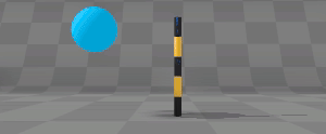
Static Colliders¶

Use the Colliders object list to add static meshes to the environment.

These meshes are converted to static rigid bodies and used as obstacles for dynamic objects. They share friction and restitution values with dynamic bodies for consistent behavior.

To speed things up you can create low poly poly meshes to use as colliders. These can be skinned, deformed or shrinkWrapped to the original mesh if needed.

You can use 3 types of static colliders:

Trimesh - this mode is the default, and uses all triangles from the provided mesh for collision detection, with full support of indentations\convex shapes and even holes. However it's more expensive than Convex to calculate, and it's performance heavily depends on how many triangles are in the mesh. Use it with meshes with concavities (like stairs) or holes (like a donut shape). It is recommended to use lower poly versions of existing meshes to be used as colliders if you need to speed up the simulation.
Convex - this mode uses only convex shapes for collision detection. This means that it can't handle concavities or holes, but it's much faster than Trimesh mode. Use this mode with simple convex objects.
Voxbox - this mode creates a grid of box colliders, it's like voxelizing the mesh (like minecraft world). It's slower than Trimesh or Convex for low and mid poly objects, but it's performance scales better with the mesh density. Use this mode when you need to simulate collisions with high detail meshes. It supports concave meshes just like Trimesh. On lower quality settings it can result in jagged edges on collision surface.

Voxbox is the only mode that has some settings:

Grid - controls voxel resolution, i.e. how many cells the mesh’s bounding box is divided into per axis during voxelization. Higher values = finer detail.
Max boxes - Maximum amount of voxels to use in collider.

Each collider shape has a Deformable checkbox. This checkbox enables or disables support for deformable colliders. When enabled, the shape of the object is queried from Maya every frame, and the collider shape is updated. Disable if your colliders are not moving and not deforming to speed up the simulation.